In my last post I discussed different integration methods using a body orbiting its parent as an example. In this post, I want to shift to focus to how orbits actually work, and give you a look into how you might implement orbits analytically.
In this series of posts, we will exclusively look at two-body systems. That means we have a larger body (the primary) with a smaller body (the satellite) orbiting around it. This is already a gross simplification of reality: a satellite orbits a primary because of the gravity the primary exerts on the satellite. The satellite is generally much smaller, but it does also exert gravity on the primary. When two bodies are in orbit, they are in fact both rotating around a central point, their shared center of mass.
The bigger the ratio between the masses of the bodies, the smaller the effect on the primary. In the case of the Earth-Moon system for example, Earth is so much more heavy than the Moon, that the center of mass of the Earth-Moon system is very close to the center of mass of Earth itself. We can thus approximate the orbit of the Moon around Earth by assuming the Moon does not contribute to the center of mass of the system.
For these posts, we won't be going as far as detangling Einstein's laws of relativity, and so we will be looking at Newtonian graphics. We will always express the position of the satellite assuming the primary is in the origin of our coordinate system.
Circular orbit
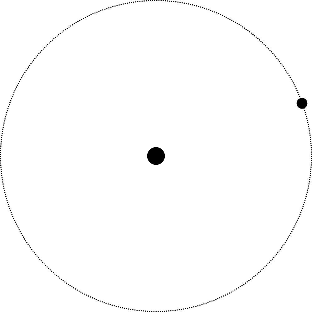
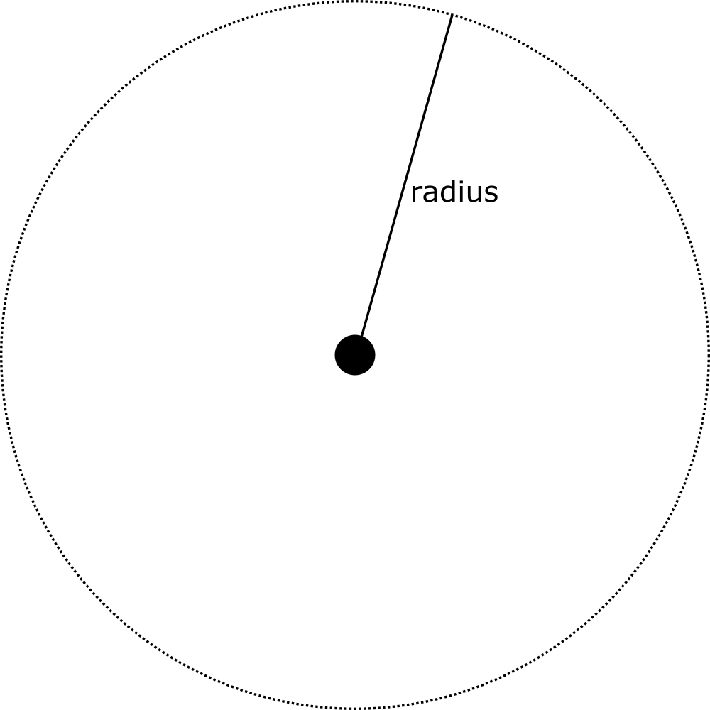
In the simplest case, the satellite moves in a perfect circle around the primary at a distance $r$.
If we wanted to represent the position of the satellite over time, we could make use of the sine and cosine functions.
$$\begin{pmatrix}x \\ y\end{pmatrix} = r \begin{pmatrix}\cos \theta \\ \sin \theta\end{pmatrix}.$$
Here $\theta$ is the angle of the satellite with the x axis of our coordinate system at any point in time. What remains is determining how this angle changes over time.
In the case of a perfectly circular orbit, the force pulling the satellite towards the primary (gravity $F_G$) is equal to the force trying to push the satellite away from it (centripetal force $F_c$). By putting the functions for both these forces on either side of the equals sign, we can derive the orbital velocity at a certain distance $r$:
$$F_G = \frac{G \cdot M_{s} \cdot M_{p}}{r^2} = \frac{M_s \cdot v^2}{r} = F_c.$$
Here $G$ is the gravitational constant. The nice thing about writing games is that we can choose the gravitational constant to be anything we want, even 1. $M_s$ is the mass of the satellite, and $M_p$ the mass of the primary, which we'll start denoting with $M$ going forward, as $M_s$ cancels out on both sides of the equation. Again, when writing games, you can just choose these values to be whatever you want. Since functions will (almost) always have $GM$ as a single clause, it's not a bad idea to choose $G$ to be 1 to simplify some of your logic. Often, the term $GM$ is simplified and denoted as $\mu$.
Let's cross out the parts of the equations we can:
$$\frac{G \cdot M}{r} = v^2.$$
This leads us to the following function for the orbital velocity of a circular orbit.
$$v = \sqrt{ \frac{GM}{r} }.$$
We can transform the actual velocity into an angular velocity $\omega$ as well, which gives us the following function:
$$\omega = \sqrt{ \frac{GM}{r^3} }.$$
Finally, transforming this into code (assuming $G=1$) is straightforward:
void Init() {
    theta = 0;
    radius = (primary.Position - position).Length;
    angularVelocity = Math.Sqrt(primary.Mass / (radius * radius * radius))
}

void Update(float elapsedSeconds) {
    theta += elapsedSeconds * angularVelocity;
    position = radius * new Vector2(Math.Cos(theta), Math.Sin(theta));
}
Position as a function of time
The function and code above calculates our orbital position incrementally. We keep track of our current angle, and each frame increment that. Another way to represent orbits though is as a function over time. For circular orbits, we know that our angular velocity over time is a constant function:
$$\omega(t) = \sqrt{ \frac{GM}{r^3} }.$$
Our angle over time is our angular velocity multiplied by the total time that has passed:
$$\theta(t) = t \cdot \omega(t).$$
Since we know how to transform $\theta$ into an actual position, we now have a function that gives the position at any given time:
$$\begin{pmatrix}x \\ y\end{pmatrix}(t) = r \begin{pmatrix}\cos ( \theta(t) ) \\ \sin ( \theta(t) )\end{pmatrix}.$$
Translating this into code is left as an exercise to the reader.
Conclusion
As you can see, the math for circular orbits works out pretty nicely. This is not the case when we start pulling in a third dimension, or if orbits stop to be perfectly circular. We'll be looking at those in future posts.