Introduction
Last time, we looked at how we can express elliptical orbits analytically. The problem is that to get the velocity on any point of the elliptical orbit, we need to solve an equation - Kepler's equation - which has no closed form solution.
While Kepler's equation doesn't have a nice direct solution, it does have a different nice property: numerical attacks work pretty well for it. That means we can use some of our knowledge about dealing with hard analytical problems on this single equation.
Fixed point iteration
Let's look at Kepler's Equation again:
$$E - e \sin{E} = (t - t_\text{per}) \cdot n.$$
We can rearrange this slightly to turn it into a more common form:
$$E = e \sin{E} + (t - t_\text{per}) \cdot n.$$
Remember that $E$ is the value we're trying to solve for. If only we knew the value of $e \sin{E}$ we could solve this equation!
The first thing we can try is falling back on the most rudimentary of solving methods: guessing. If we have a guess for $E$, we can try filling it in on the right-hand side of the equation. This gives us a new value for $E$ on the left which is a better guess than our previous one. For example, let's start by guessing $0$. The next guess will be $E_1$ and is given by:
$$E_1 = (t - t_\text{per}) \cdot n.$$
Choosing $0$ as first guess causes the first term to be eliminated from the equation, leaving a pretty straightforward thing to calculate. If your eccentricity $e$ is close to zero - that is, if your orbit is near circular - the first part of the equation will not dominate the result either way. That makes sense, because with just some slight changes in notation, the equation above is just the equation for angle with the periapsis over time in a circular orbit:
$$\theta(t) = (t - t_\text{per}) \cdot \omega.$$
Since we're trying to solve our equation for actual elliptical orbits, we're not done yet. We can take our initial guess and fill it into Kepler's equation to get a better guess. In general:
$$E_{n+1} = e \sin{E_n} + (t - t_\text{per}) \cdot n.$$
Given enough iterations, this will converge to the actual solution for $E$. The number of iterations you need depend on your eccentricity $e$. For high eccentricities, you will need many iterations to find a close enough solution. This is the original solution Kepler used in the 17th century.
The code for this is relatively straight-forward:
double SolveKeplerThroughIteration(double e, double t, double tPer, double n)
{
    const numIterations = 30; // Change depending on expected eccentricities.

    // Pre-calculate the current mean motion because it doesn't change.
    var M = (t - tPer) * n;
    var E = 0;

    for (int i = 0; i < numIterations; i++)
    {
        E = e * Math.Sin(E) + M;
    }

    return E;
}
Instead of using a fixed number of iterations, you could also consider iterating until you find the difference between $E_n$ and $E_{n+1}$ to be small enough to live with. However, note that this potentially introduces a variable cost in your game update loop, so bounding the number of iterations is always a good idea.
Newton's method
The fixed point iteration method is easy to implement and generally returns accurate results relatively quickly. It is a pretty dumb way to iterate though. This is something that is solved in Newton's method. It still starts with a guess that we will use to get closer to the final answer, but the choice of the next guess is done differently.
We could rearrange Kepler's equation once again.
$$e \sin{E} + (t - t_\text{per}) \cdot n - E = 0.$$
The left part could be considered a function $f(E)$. The values $E$ for which a function $f(E)$ is zero are called the roots of the function. In this case, finding the root of $f(E)$ gives us a solution for Kepler's equation.
The reason we're taking this roundabout approach to solving Kepler's equation, is because finding roots for functions is a problem mathematicians have been trying to solve for a long time, and there are ways to do that in a smarter way than trying out arbitrary values. One of these methods, and probably the most famous of these approaches, is Newton's method. This method also works with an iterative approach, but the different iterations $E_n$ are defined in a different way.
Assuming an initial guess $E_0$, the following guesses are given by
$$E_{n+1} = E_n - \frac{f(E_n)}{f'(E_n)}.$$
Newton's method uses the rate of change, given by the derivative, to make more educated guesses as to where the function is going. For our version of Kepler's equation, we get the following expression for $E_{n+1}$:
$$E_{n+1} = E_n - \frac{e \sin{E} + (t - t_\text{per}) \cdot n - E}{e \cos{E} - 1}.$$
For most eccentricities $e < 0.8$, $E_0 = t - t_\text{per}$ is a good starting point. If your eccentricities go beyond $0.8$, you can use $E_0 = \pi$.
Translating this into code doesn't look too different from the code above.
double SolveKeplerThroughNewtonIteration(double e, double t, double tPer, double n)
{
    const numIterations = 30; // Change depending on expected eccentricities.

    // Pre-calculate the current mean motion because it doesn't change.
    var M = (t - tPer) * n;
    // Make an initial guess based on the eccentricity of the orbit.
    var E = e > 0.8 ? Math.PI : M;

    for (int i = 0; i < numIterations; i++)
    {
        var numerator = e * Math.Sin(E) + M - E;
        var denominator = e * Math.Cos(E) - 1;
        E = E - numerator / denominator;
    }

    return E;
}
Another advantage of this approach is that you are trying to get a function as close to $0$ as possible, which makes it easy to change the exit condition of your loop based on the current output. Just fill in your current $E_n$ in $f$ and check if it's smaller than your desired difference.
Back to the physical world
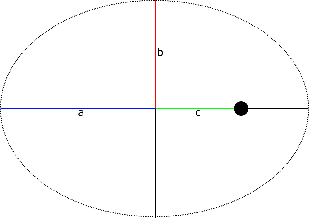
Now that we have ways to solve for $E$, we can turn back to our physical world and attempt to turn this into a position we can use to update and/or draw our game world. In the previous post, we established that the position on an ellipse is given by
$$\begin{pmatrix}x \ y\end{pmatrix} = \begin{pmatrix}a \cos E \ b \sin E\end{pmatrix}.$$
This position is relative to the centre of the ellipse, which is not the same as the position of our primary, which is located in one of the foci of our ellipse.
In the next post I'll show how the math can be made to work out, and we'll also introduce a third dimension to talk about inclined orbits.
Closing words
In this post we looked at two ways to solve Kepler's equation, which is needed to keep track of orbits in an analytical way. The reason we started with the analytical approach was to avoid numerical errors, so falling back on a numeric approach for elliptical orbits seems to to defeat the point. However, for orbits we tried avoiding the numerical approaches for a very particular reason: they make stable orbits deviate and either diverge or converge over time. This is because the outcome of our numerical approach is used in the following frame, so our error adds up. For elliptical orbits on the other hand, we use numerical approaches to turn our source truth variables into something we can display, but the errors that slip in don't propagate to following frames.
There may still be floating point imprecision errors in keeping track of the current time, but the only problem that will introduce is that our satellite may not quite move at the right velocities around the orbit any longer. It will still be in one of the positions on the correct orbit though, and this orbit will never deteriorate. For many games, keeping the orbits constant is important, and this solution solves that problem.