It is not uncommon for games to contain some form of game physics. The most common - and probably most intuitive - of those, is gravity. In a simplified situation where we ignore air resistance, gravity applies a constant acceleration to an object (no matter its mass), which increases its downward velocity.
Gravity can also occur over longer distances: between orbiting bodies. I want to take orbits as an example today, since they lend themselves to some nice simplifications. When we talk about orbits, we often talk about a small body (the satellite) orbiting a static large body (the primary).
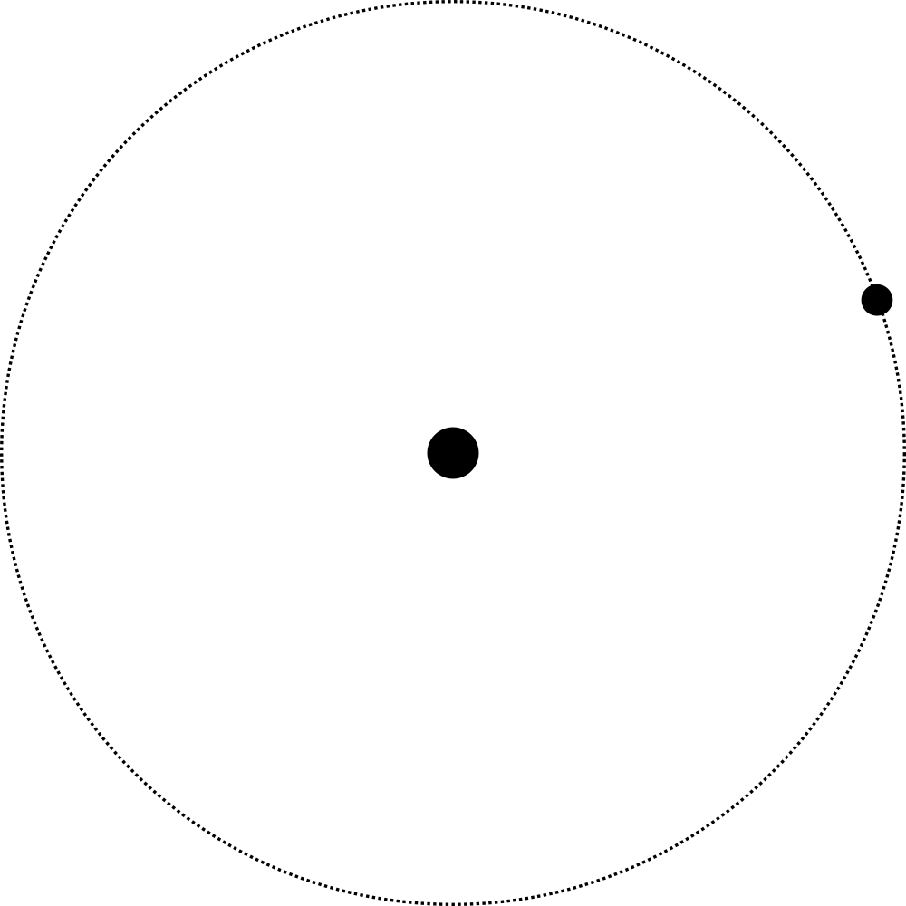
The principle of an orbit is the same as normal gravity, but we need to be a bit more careful about the direction of our vectors. The primary pulls on the satellite, causing an acceleration that's orthogonal to the satellite's current velocity. The satellite's velocity is therefore altered so its trajectory curves towards the primary, but never enough to fall down.
The problem
In games, we generally don't simulate constant acceleration. Instead, we update the state of our universe in fixed time steps. The code for updating the satellite could look something like this:
void Update(float elapsedSeconds) {
    velocity += acceleration * elapsedSeconds;
    position += velocity * elapsedSeconds;
}
The exact orbiting speed depends on the distance, the bodies' masses and the gravitational constant, which we can ignore. Instead we just choose an orbiting speed. In fact, we can just always assume that the current velocity vector is the orthogonal of the vector pointing from the satellite to the primary. In 2D, that makes our code:
void Update(float elapsedSeconds) {
    toPrimary = (primary.Position - position).Normalized();
    // We use the clockwise orthogonal as velocity direction,
    // causing a counter-clockwise orbit.
    velocity = speed * new Vector2(toPrimary.Y, -toPrimary.X);
    position += velocity * elapsedSeconds;
}
The exact velocity calculation does not matter for our topic today, in so far as that it is the derivative of the position as a function in time. This means that we can express the calculation above as mathematical equation too:
$$p(t_0 + \epsilon) = p(t_0) + \epsilon \cdot \dot p (t_0).$$
The position at some time $t_0 + \epsilon$ for the elapsed time $\epsilon > 0$ is the position at $t_0$ plus the velocity at $t_0$ multiplied by the elapsed time.
What we have actually done here is applying the Euler method to use a differential equation. In each step, we approximate the movement of the satellite that happened in the period between last frame and the current. We do this by using a constant velocity during this time period. However, in reality, the velocity constantly changes to arc the object towards the primary. We end up changing the position of the satellite slightly further away from the primary than the expected order.
In most cases, this may not matter than much. However, if your game expects orbits for example to be stable, you'll find that if you leave the game running long enough, satellites will slowly move away further and further from their primary. You can see this in the image below:
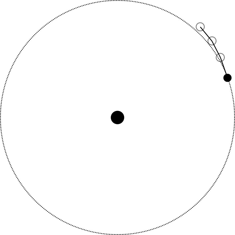
In the animation above, the speeds and time steps have been exaggerated to highlight the error. In normal circumstances the error will be much less egregious, but it is there nonetheless. Let's look into a few ways we can fix this.
Smaller steps
When we talk about the speed of a game, we usually quickly arrive at talking about FPS - frames per second. FPS is inherently a graphics concept, and talks about how often we can render the game to the screen per second. Often FPS is linked to the numbers of updates per second - UPS. It is not uncommon for games to render more frames per second than the refresh rate of the monitor can handle, especially in games that are fast-paced, to reduce the input lag for its players.
If we have a game where our rendering takes significantly slower than our updating, it doesn't make much sense to link those two together. In general, the major bottleneck of the rendering is the GPU, while the updating is mostly limited by the CPU resource. By separating the update loop from the rendering loop, we can try to squeeze as many update cycles as possible out of the CPU. That way we reduce the time steps, and the error over time.
Sometimes it's not possible or practical to separate the actual loops, but that doesn't prevent us from doing more update cycles than rendering cycles. When we have a game running at 60 FPS, we can always decide to split the time per frame in two, and do two update cycles with half the time step every frame. This means we are effectively updating at 120 UPS. This has the drawback that if the update cycle takes too long, we can't keep up the 60 FPS, and we'll slow down the rendering as well.
Reducing the time deltas will reduce the error build-up over time. This makes sense, since mathematically taking the limit of the time delta approaching 0 gives us the actual result we want. However, getting a small delta is not always possible, especially if we keep in mind that less powerful machines may have less UPS than a massive gaming rig. Let's look at some mathematical tricks that we may use instead.
Midpoint method
The source of the error in the Euler method is that we look at the derivative of the position (which is the velocity) at $t_0$. The velocity changes over time, and this is not accounted for. Instead of looking at the derivative at $t_0$, we can look at the derivative at $t_0 + \epsilon / 2$. The idea is that instead of assuming that our velocity over time can be approximated by a constant velocity, we assume that our acceleration (the change in velocity) can be approximated by a constant acceleration instead. By looking at the velocity at $t_0 + \epsilon / 2$, the intuition is that we take the average velocity over our time delta, which gives a closer approximation. In a mathematical expression, this is expressed as:
$$p(t_0 + \epsilon) = p(t_0) + \epsilon \cdot \dot p (t_0 + \frac{\epsilon}{2}).$$
The problem is that we don't know the value of $\dot p (t_0 + \epsilon/2)$. However, we can always use our original trick of using the Euler method to find $p (t_0 + \epsilon/2)$ and calculate the derivative in that point.
This method is named the midpoint method after the fact that we are looking at the midpoint of our time segment to get the derivative to use. Let's take a quick look at how this could look in code:
void Update(float elapsedSeconds) {
    var velocityAtCurrent = velocityAt(position);
    var midpoint = position + velocityAtCurrent * elapsedSeconds * .5f;
    var velocityAtMidpoint = velocityAt(midpoint);
    position += velocityAtMidpoint * elapsedSeconds;
}

Vector2 velocityAt(Vector2 pos) {
    toPrimary = (primary.Position - pos).Normalized();
    return speed * new Vector2(toPrimary.Y, -toPrimary.X);
}
We see that we need to do roughly double the calculations, but we get more precision in return.
Heun's method
We have looked at the velocity at $t_0$ and $t_0 + \epsilon / 2$, but what about the velocity at $t_0 + \epsilon$? If we use the velocity at $t_0$, we get a result (this is the Euler method), and if we use $t_0 + \epsilon$ we get a different result. It is very likely that our actual result is somewhere between these two. Heun's method is based on this. It uses the Euler method to calculate a first approximation. Then we calculate the velocity at this new point, and use it to make another approximation. We average our two approximation and use that as a final solution. This is a bit easier to express in code than in math, so let's start there:
void Update(float elapsedSeconds) {
    var velocityAtCurrent = velocityAt(position);
    var eulerPosition = position + velocityAtCurrent * elapsedSeconds;
    var velocityAtEulerPos = velocityAt(eulerPosition);
    var heunPosition = position + velocityAtEulerPos * elapsedSeconds;

    position = .5f * (eulerPosition + heunPosition);
}

Vector2 velocityAt(Vector2 pos) {
    toPrimary = (primary.Position - pos).Normalized();
    return speed * new Vector2(toPrimary.Y, -toPrimary.X);
}
Below is an attempt to describe this mathematically:
$$
\begin{aligned}
p_{\text{Euler}}(t_0 + \epsilon) & = p(t_0) + \epsilon \cdot \dot p (t_0) , \
p_{\text{Heun}}(t_0 + \epsilon) & = p(t_0) + \epsilon \cdot \dot p_{\text{Euler}} (t_0 + \epsilon) , \
p(t_0 + \epsilon) & = \frac{p_{\text{Euler}}(t_0 + \epsilon) + p_{\text{Heun}}(t_0 + \epsilon)}{2} .
\end{aligned}
$$
Analytical
We can also take a different approach entirely. Instead of approximating our physics, we could use the exact analytical solution as well. For a circular orbit, we just need to be able to describe a point moving along a circle, which is fairly straightforward. For eccentric orbits things get a bit more complicated, and we'll discuss this in a follow-up post.
In general, analytical solutions are impractical. While we may be able to calculate simple systems (two body orbital systems, a single falling object), it becomes impractical for larger problems.
Closing words
Integration methods have the problem that they accumulate errors. The small error we introduce in one frame will live on in all future frames of our simulation. In orbital mechanics, this often leads to drift, and causes stable orbits to eventually become unstable. In many practical cases, the physical simulations don't take long enough, or the effects aren't noticeable enough that we need to worry about it, but in some cases we need to do a bit of extra work to make things look right.
Orbits are a feeble thing, as they are easy to make unstable with an accumulated error. That's why we will spend the next few blog posts picking apart the math behind orbital mechanics, and try to build an implementation of orbits that can keep running for an indefinite amount of time.